Excel 2007中数据需要透视表建立、刷新、统计数据的方法，今天，小编就来告诉大家怎么使用滤镜方法操作。

工具原料：excel 2007

excel 2007滤镜方法步骤如下：

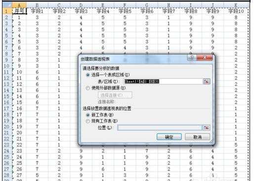
打开要统计的数据表格，选中数据表格中任意一个有数据的单元格，把软件的注意力引过来→插入→数据透视表→确定。 (软件会默认框选整个表格的数据，默认数据透视表在新的工作表中显示)

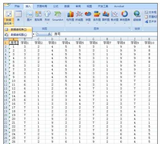
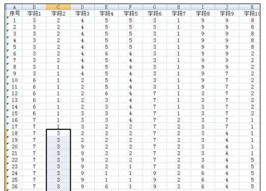
序号列是文本格式，且不重复，可以用来计数(有多少个序号，就有多少行数据)，现在统计下字段1中各种数值出现的情况：

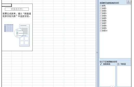
用鼠标将“序号”拖拽至右下角计数框中

→将“字段1”拖拽至“行标签”中

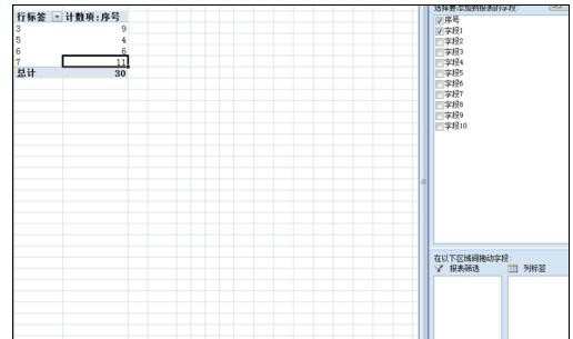
→结果显示：字段1取值有3、5、6、7四种情况，出现频次分别为9、4、6、11，共30个取值，见下图：

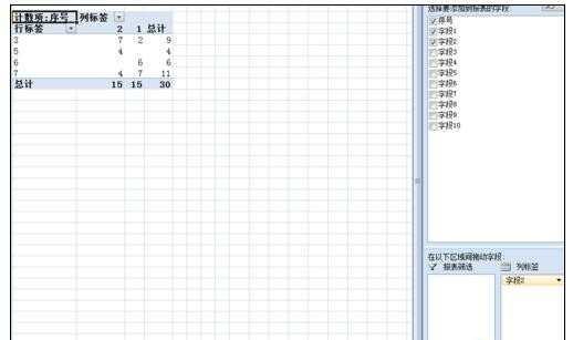
再来看看字段2与字段1取值情况：

将字段2拖拽至“列标签”，结果显示：字段2取值仅1、2两种情况，且字段1取值为3时，字段2有7个数据取值为2，2个取值为1;字段1取值为5时，字段2只有取值为2一种情况，共4个……

详见下图：

返回数据表，更新部分数据，字段2部分取值改为3，如下图

回到透视表，发现统计结果没有变化，这是不能用的。如何更新?

鼠标右击统计结果表格→刷新

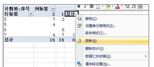
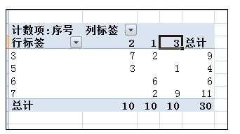
结果变化了：