INDEX函数是返回表或区域中的值或对值的引用，应该怎么在excel表格中使用该函数呢?下面就跟小编一起来看看吧。

excel表格使用INDEX函数的步骤

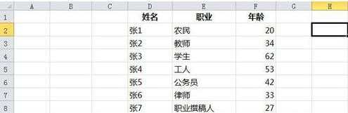
举例1：在H2单元格中返回数组(D2：F11)中第3行、第3列的值。

如下图所示：

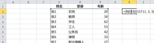
在H2单元格中输入“=INDEX(D2：F11, 3, 3)”, 然后单击“Enter”键：

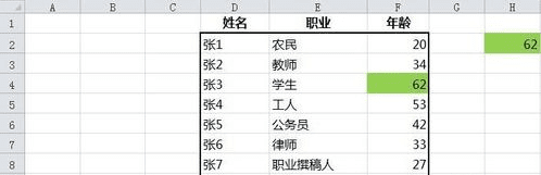
最后H2单元格中返回的值为“62”，“62”是我们所选区域(D2：F11)的第3行、第3列的值，而不是整个Excel的第3行、第3列的值：

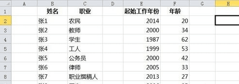
接下来介绍引用形式的使用方法

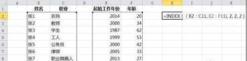
举例2：在H2单元格中返回两个数组区域(B2：C11)和(E2：F11)的第二个区域的第2行、第2列的值。

在H2单元格中输入“=INDEX((B2：C11, E2：F11), 2, 2, 2)”, 然后单击“Enter”键：

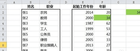
最后H2单元格中返回的值为“34”，“34”是我们所选区域(B2：C11, E2：F11)的第2个区域(E2：F11)第2行、第2列的值

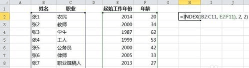
将第7步中H2单元格中的输入“=INDEX((B2：C11, E2：F11), 2, 2, 2)”改为“=INDEX((B2：C11, E2：F11), 2, 2)”，查看一下省略area_num的结果：

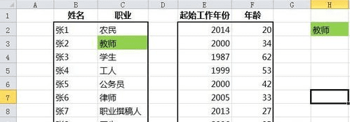
最后H2单元格中返回的值为“教师”，“教师”是我们所选的第1个区域(B2：C11)的第2行、第2列的值，由此可见当省略area_num时，其值默认为1