很多人在财务工作的的小伙伴一般都会用到excel2013软件，对于财务的朋友来说，制作数据透视表是很常用也很实用的excel技巧，下面是小编整理的excel2013制作数据透视表的方法，供您参考。

excel2013制作数据透视表的方法

首先打开需要制作数据透视表的excel文档

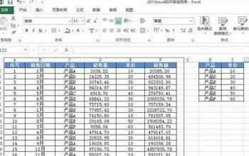
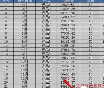
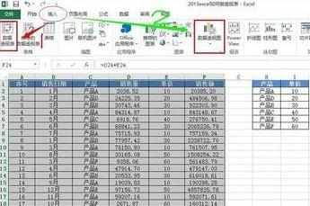
以如图所示为例，选取选择A1：F24区域(表头也需要选取)

点击“插入”→“数据透视图”(有两种方法，以第一种为例)

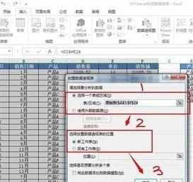
弹出“创建数据透视表”窗口，这里可以可以重新选择或更好数据源区域以及什么地方生成数据透视表，这里默认为例，点击确定

最后在新表位置生成了一个数据透视表

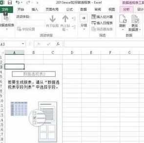
在右侧弹出的就是数据透视表工具栏中，可以看到源数据表头的各个字段，这个时候就可以往右下角区域拖拽字段进行透视展现

例如我要知道各种产品的销售量汇总，我先把“产品”拖到“行”区域，然后把“销售量”拖到“值”区域，这样一个基于产品统计销售量的透视表就生成了。

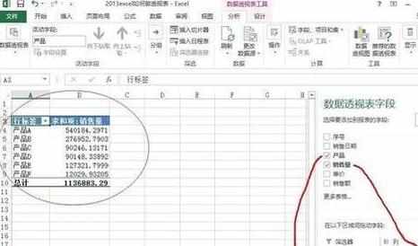
提示：可以同时选择两个列维度或两个行维度

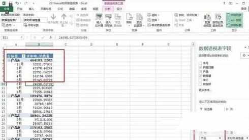
例如： 行区域选择了日期和产品两个维度查看 销售量，如图所示