想要在excel中使用匹配函数，如何使用呢，今天，小编就教大家如何使用匹配函数的方法。

Excel中匹配函数的使用方法如下：

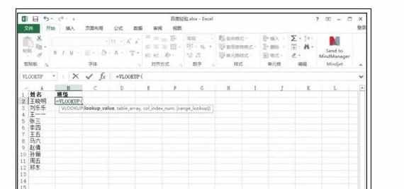
打开需要设置的excel文档，这里以如图所示Excel为例。

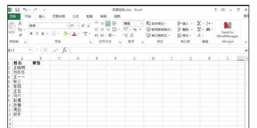
这里需要在另一个表中找出相应同学的班级信息。

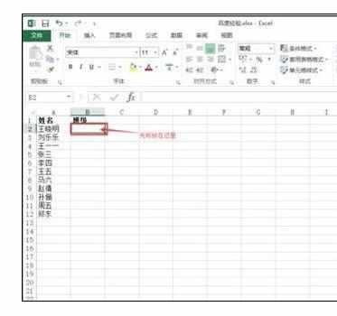
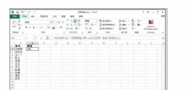
如图所示，将光标放在要展示数据的单元格中。

然后在单元格中输入“=vl”，会自动提示出VLOOKUP函数，双击蓝色的函数部分。

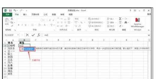
可以看到单元格中出现VLOOKUP函数。

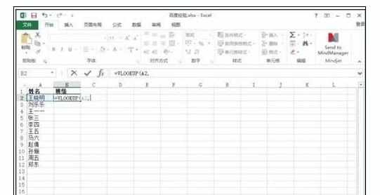
选择第一列中需要匹配数据的单元格，选中一个就可以，然后输入英文状态下的逗号“,”。

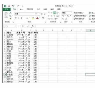
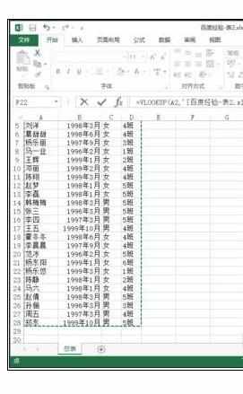
然后返回到第二张表“百度经验-表2”，选中全部数据。

需要“百度经验-表2”中第四列的班级信息，所以在公式中再输入“4,”(逗号是英文的)。

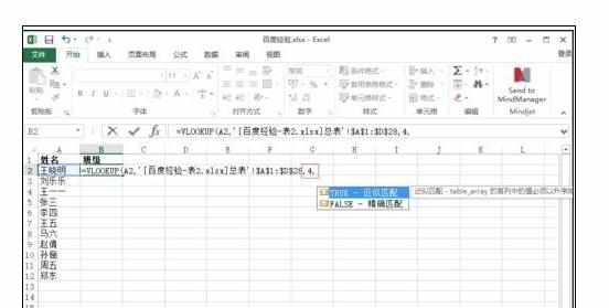
回车，展示数据，如图所示即为效果。

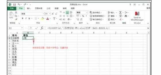
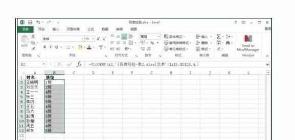
要把一列中的数据都匹配出来，只需要按如图所示操作。

如图所示为最后的效果。