在用Excel制作图表时，如果纵轴系列过多会导致在图形上观察数据的不便。如何利用函数公式和定义名称来实现可以用鼠标点选逐个显示系列数据的动态图表。今天，小编就教大家在Excel表格中制作动态图表的操作方法。

Excel表格中制作动态图表的操作步骤如下：

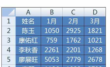
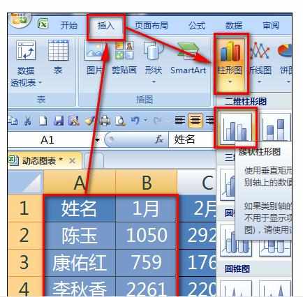
1、首先看一下原始数据，A列是姓名，B列及以后是各月份的销售数据。本例显示1到3月的销售数据情况，实际情况可能有更多列。

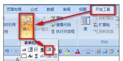
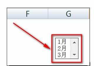
2、点击功能区的【开发工具】-【插入】-【列表框】。

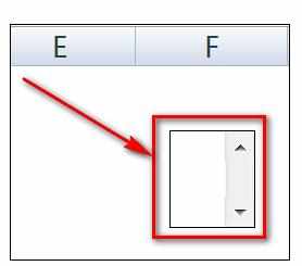
3、用鼠标在工作表上用左键画出一个列表框控件。

4、在E2:E4输入原始数据各月份的标题，本例是1月、2月和3月。

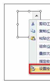
5、选中列表框，鼠标右键，选择【设置控件格式】。

在【控制】选项卡进行如下图设置：

【数据源区域】选择刚才输入的E2:E4;

【单元格链接】选择E1。

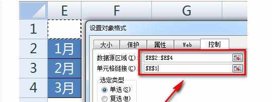
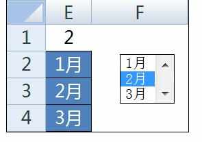
点击【确定】按钮后列表框中就显示了E2:E4范围数据。当选择不同的内容时在E1单元格将返回选择的内容是列表框中的第几项。

点击功能区上的【公式】-【定义名称】。

定义一个名称为“月份”，引用位置处输入公式：

=INDEX($B$2:$D$7,,$E$1)

知识点说明：INDEX的作用是从$B$2:$D$7中选取第E1单元格数值的列。如果E1是2，就返回$B$2:$D$7区域的第2列数据，也就是C2:C7。

选中AB两列数据，点击【插入】-【柱形图】。

稍微调整一下插入图表的格式，并将列表框挪到图表右上角位置。

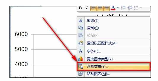
在图表上鼠标右键，选择【选择数据】。

选中“1月”这个系列，并点击【编辑】。

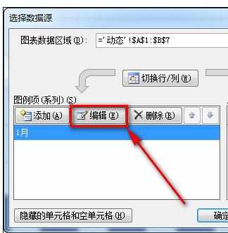
输入一个系列名称，然后将【系列值】改成刚才定义的名称，然后点击【确定】按钮后，动态图表就制作完成了。

我们分别用鼠标点选列表框中的不同项目，图表就会返回不同月份的数据。