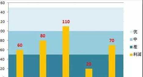
这是很多excel图表用户很想实现的一个功能。它就是图表分层填充颜色。如你想在excel图表中，从下至上分三种蓝色作为背景，分别显示差(<50)、中(<100)、优(<150)3个档次。要怎么做呢?下面小编来告诉你吧。

excel图表分层填色的步骤：

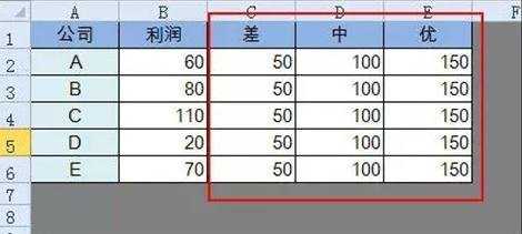
设计源数据表，把50、100和150输入到CDE列中。

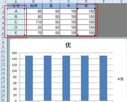
选取A列和E列，插入图表 - 柱状图

在柱子上右键单击 - 设置数据系列格式，把系列重叠调整最大，分类间距调整为0%。

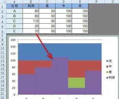
依次复制D、C、B列数据，粘到图表上，结果如下图所示。

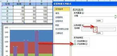
选取利润系列并单击右键 - 设置数据系列格式 - 把坐标轴设置为次坐标轴，然后把分类间隔调整为20%

在左侧坐标轴上右键 - 设置坐标轴格式 - 最大值150。

然后再把次坐轴标的最大值也设置为150，设置完成后效果：

选取次坐标轴，按delete键删除，然后分别修改各个系列柱子的颜色，最后添加上数据标签，最后完成效果如下图所示。

excel图表怎么分层填色相关文章：

1.Excel制作图表教程

2.excel怎样设计图表

3.怎么在excel2013中使用推荐的图表

4.怎么在excel2013中制作组合图表

5.怎样制作EXCEL图表

6.excel怎么制作统计图表