Excel中MATCH函数是一个很强大的辅助函数，那么excel表格中怎么使用?下面就跟小编一起看看吧。

excel表格使用match函数的步骤

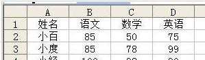
首先点击打开需要编辑的excel表格

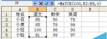
如图所示表格，选择B7单元格，输入“=MATCH(100，B2：B5，0)”,按回车，显示“3”

在“B2：B5”区域内查找一个等于“100”的数值为第几个，按顺序找到B4单元格的数值为“100”，B4在“B2：B5”区域内排第3，所以显示“3”

选择C7单元格，输入“=MATCH(80，C2：C5，1)”，回车显示“2”

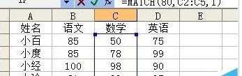
在“C2：C5”区域内查找小于或等于“80”的数值，按顺序找到C2：C3单元格的数值都小于“80”，选择其中最大的数值，即C3的数值，C4在“C2：C5”区域内排第2，所以显示“2”

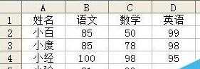
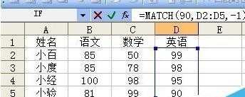
D7单元格，输入“=MATCH(90，D2：D5，-1)”，回车显示“4”

在“D2：D5”区域内查找大于或等于“90”的数值，按顺序找到D2：D5单元格的数值都大于“90”，选择其中最小的数值，即D5的数值，D5在“D2：D5”区域内排第4，所以显示“4”

excel表格match函数相关文章：

1.怎么在excel中使用MATCH函数

2.excel中match函数的使用教程

3.excel中match函数的用法

4.excel函数match的使用教程